%matplotlib inline
from __future__ import division

import numpy as np
import matplotlib
from datetime import datetime

#Using https://dtcooper.github.io/python-fitparse/ to parse the fit file
from fitparse import FitFile
#These two help parse the tcx files not needed if only doing fit files
from xml.dom.minidom import parse
import xml.dom.minidom

#Plotly used for interactive plots for comparison 
from plotly.offline import download_plotlyjs, init_notebook_mode, plot, iplot
from plotly.graph_objs import Scatter, Figure, Layout
init_notebook_mode(connected=False)

#LOAD AN EXAMPLE FIT FILE
fit = '2018-03-11-020856-ELEMNT BBCD-22-12.fit'

#LOAD AN EXAMPLE TCX FILE
tcx = 'rob0-2020-05-12-gendarme-1-80858341.tcx'

Load and parse an example fit file

#LOAD FIT FILE AND PARSE
fit_watts = []
fit_time = []

fitfile = FitFile(fit)
# Get all data messages
count = 0
for record in fitfile.get_messages('record'):
    # Process all records
    for record_data in record:
        
        if record_data.name == 'power' and record_data.value: 
            fit_watts.append(record_data.value)
        elif record_data.name == 'power':
            fit_watts.append(0)
            #continue
        if record_data.name == 'timestamp': fit_time.append(record_data.value)
        
trim = len(fit_time)-len(fit_watts)
if trim > 0:
    fit_time = fit_time[:-trim]

t = (fit_time[-1]-fit_time[0]).seconds/3600.

EXAMPLE OF A SIMPLE STEADY STATE SOLUTION

You only need the average power

# Define the basic constants / assumed values
g = 9.81         #gravity in m/s^2
m = 79.4         #rider + bike mass in kg
Crr = 0.005      #approximate rolling resistance
CdA = 0.324      #approximate CdA in m^2 - hands on hoods elbows bent
Rho = 1.225      #air density sea level STP

#Calculate the average power from the fit file
p = np.average(fit_watts)  

#This calculates the steady state velocity in m/s and converts to MPH
n = (((((8*g**3*Crr**3*m**3+27*CdA*Rho*p**2)/(CdA*Rho))**0.5+p*5.196)/(Rho*CdA))**(1/3.0))**2*Rho*CdA-2*m*Crr*g
d = 3**0.5*Rho*CdA*(((8*g**3*Crr**3*m**3+27*CdA*Rho*p**2/(CdA*Rho))**0.5+p*5.196)/(Rho*CdA))**(1/3.0)
v = n/d*2.23694   

print "Average Power {:0.1f} - Average Speed: {:.1f} mph - Time: {:.1f} hours - Distance: {:.1f} miles".format(p,v,t,(v*t))

Average Power 196.1 - Average Speed: 20.8 mph - Time: 1.5 hours - Distance: 31.2 miles

EXAMPLE OF FORWARD INTEGRATION

And comparison with the steady state values

g = 9.81         #gravity in m/s^2
m = 79.4 + 1     #rider + bike mass in kg with 1kg more representing the rotational intertia
Crr = 0.005      #approximate rolling resistance
CdA = 0.324      #approximate CdA in m^2 - hands on hoods elbows bent
Rho = 1.225      #air density sea level STP
dt=1  #time step from the fit/tcx files

Calculating the speed through forward integration

• Starting with a iniiial velocity of 0 mph
• Calculate the speed at the next time step using the equation below
• Update the initial velocity with the current velocity and repeat

#This will calculate the speed at each time step
speed = []                      #list to hold the second by second speed data
Vi = 0                          #initialize the starting speed at 0  
for p in fit_watts:             
    #for each time step do the following equation to determine the speed for the next second
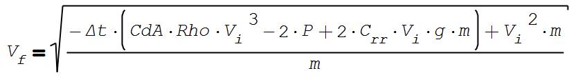
    Vf = ((-dt*(CdA*Rho*Vi**3-2*p+2*Crr*Vi*g*m)+Vi**2*m)/m)**.5
    speed.append(Vf* 2.23694)   ##convert from m/s to MPH for display, add this new speed to the list
    Vi = Vf                     #update the current speed - it will be the start for the next calculation
    
v = np.average(speed)           #get the average speed     
t = (fit_time[-1]-fit_time[0]).seconds/3600.   #calculate the length of the ride in hours

The next cell calculates the speed and distance using a steady state model and the average power - one step but less accurate

p = np.average(fit_watts)
n = (((((8*g**3*Crr**3*m**3+27*CdA*Rho*p**2)/(CdA*Rho))**0.5+p*5.196)/(Rho*CdA))**(1/3.0))**2*Rho*CdA-2*m*Crr*g
d = 3**0.5*Rho*CdA*(((8*g**3*Crr**3*m**3+27*CdA*Rho*p**2/(CdA*Rho))**0.5+p*5.196)/(Rho*CdA))**(1/3.0)
v_ss = n / d * 2.23694  #convert m/s to mph

#display the results for comparison
print "Power_Avg {:0.1f} - Speed_SS: {:0.1f} mph - Speed_Modeled {:0.1f} mph - Dist_SS: {:0.1f} miles - \
Dist_Modeled {:0.1f} miles".format(p,v_ss,v,(v_ss*t),(v*t))

Power_Avg 196.1 - Speed_SS: 20.8 mph - Speed_Modeled 20.6 mph - Dist_SS: 31.2 miles - Dist_Modeled 30.9 miles

Plot of the power (watts) and calculated speed (mph)

skip=1
iplot([{"x": fit_time[::skip], "y": fit_watts[::skip], "name": "power - watts"}])
iplot([{"x": fit_time[::skip], "y": speed[::skip], "name": "speed - mph"}])

Load and parse a tcx file

dom = xml.dom.minidom.parse(tcx)
file = dom.documentElement

tcx_watts = []
tcx_time = []

seg = dom.getElementsByTagName("ns3:Watts")
for c,item in enumerate(seg):
    tcx_watts.append(int(item.firstChild.data))
    
seg = dom.getElementsByTagName("Time")
for item in seg:
    t = item.firstChild.data
    tcx_time.append(datetime.strptime(t, '%Y-%m-%dT%H:%M:%SZ'))

Calculating the speed through forward integration

• Starting with a initial velocity of 0 mph
• Calculate the speed at the next time step using the equation below
• Update the initial velocity with the current velocity and repeat

#This will calculate the speed at each time step
speed = []                      #list to hold the second by second speed data
Vi = 0                          #initialize the starting speed at 0  
for p in tcx_watts:             
    #for each time step do the following equation to determine the speed for the next second
    Vf = ((-dt*(CdA*Rho*Vi**3-2*p+2*Crr*Vi*g*m)+Vi**2*m)/m)**.5
    speed.append(Vf* 2.23694)   ##convert from m/s to MPH for display, add this new speed to the list
    Vi = Vf                     #update the current speed - it will be the start for the next calculation
    
v = np.average(speed)           #get the average speed  
t = (tcx_time[-1]-tcx_time[0]).seconds/3600.   #calculate the length of the ride in hours

The next cell calculates the speed and distance using a steady state model and the average power - one step but less accurate

#These next four lines show the calculation for the steady state velocity from the average power
p = np.average(tcx_watts)       #calculate the average power
n = (((((8*g**3*Crr**3*m**3+27*CdA*Rho*p**2)/(CdA*Rho))**0.5+p*5.196)/(Rho*CdA))**(1/3.0))**2*Rho*CdA-2*m*Crr*g
d = 3**0.5*Rho*CdA*(((8*g**3*Crr**3*m**3+27*CdA*Rho*p**2/(CdA*Rho))**0.5+p*5.196)/(Rho*CdA))**(1/3.0)
v_ss = n / d * 2.23694              #convert the steady state velocity from m/s to MPH

#display the results for comparison
print "Power_Avg {:0.1f} - Speed_SS: {:0.1f} mph - Speed_Modeled {:0.1f} mph - Dist_SS: {:0.1f} miles - \
Dist_Modeled {:0.1f} miles".format(p,v_ss,v,(v_ss*t),(v*t))

Power_Avg 188.3 - Speed_SS: 20.5 mph - Speed_Modeled 20.1 mph - Dist_SS: 20.5 miles - Dist_Modeled 20.1 miles

Plot of Ride Power and Ride Speed

skip=1
iplot([{"x": tcx_time[::skip], "y": tcx_watts[::skip], "name": "power - watts"}])
iplot([{"x": tcx_time[::skip], "y": speed[::skip], "name": "speed - mph"}])

Alternative method

This shows each step, but has problems when Vi is zero

#This calculation is more explicit - however care must be taken when the speed is near zero
speed2 = []
Vi = 0 
for p in tcx_watts:
    Wroll = Crr*m*g*Vi           #For each time step calculate Watts lost to rolling resistance
    Wair = 1/2*CdA*Rho*Vi**3     #And the wind resistance
    Wacc = p - Wroll - Wair      #If this is positive then the bike accelerates, negative is slows down
    if Vi:                       #This is to avoid a divide by 0 error if Vi = 0
        F = Wacc/Vi              #Calculate the force 
    else:
        F = Wacc/1
    a = F/m                      #Newton's second law - we get the acceleration
    Vf = Vi + a*dt               #This calculates how much velocity changes for this time step
    speed2.append(Vf * 2.23694)  #Record the speed for this time step
    Vi = Vf                      #Update the current speed to be used in the next time step

This plot shows the results are the same

#This is a plot of the two methods - they line up as expected
iplot([{"x": tcx_time[::skip], "y": speed[::skip], "name": "method1"},
       {"x": tcx_time[::skip], "y": speed2[::skip], "name": "method2"}])